This post is part of the univariate models chapter within a larger learning series around time series forecasting fundamentals. Check out the main learning path to see other posts in the series.
The example monthly data used in this series can be found here. You can also find the python code used in this post here.
What Does Exponential Smoothing Mean?
Exponential smoothing is a family of forecasting methods that smooth out short-term fluctuations in data to reveal underlying trends or patterns. The core idea is to give more weight to recent observations and less weight to older data, which produces a “smoothed” time series with reduced noise. This makes it easier to spot patterns and predict future values.
It’s also referred to as ETS, which stands for error, trend, and seasonality. These three components are at the heart of the most advanced exponential smoothing methods. Sometimes you might also hear them be called “state space” models, since they are modeling out different states like trend and seasonality separately.
- Error (E): The unpredictable or random fluctuations (noise) around your forecast.
- Trend (T): A longer-term movement (upward or downward) observed in your data.
- Seasonality (S): Regular patterns or cycles occurring within a known fixed period (e.g., yearly, monthly, weekly).
Another component of these models is something called the level. Think of the level (sometimes called the baseline) as the smoothed estimate of ‘where we are right now’, before any trend pushes us up or seasonality ripples us up and down. Here’s how they are put together.
- Baseline right now → level
- How the baseline is moving → trend
- Repeating wiggles → seasonality
- Random noise around all that → error
Types of Exponential Smoothing
Exponential smoothing isn’t a single technique but a family that includes simple (single) smoothing, double smoothing, and triple smoothing. Each one builds on the previous to handle more complex patterns in the data:
- Simple Exponential Smoothing: Used for data with no clear trend or seasonality.
- Double Exponential Smoothing (Holt’s Linear Trend): Used for data with a trend (increasing or decreasing sales over time).
- Triple Exponential Smoothing (Holt-Winters): Used for data with both trend and seasonality (recurring seasonal patterns, such as higher sales every holiday season).
Most time series we deal with in the business have both trend and seasonality, so we’ll focus mostly on triple exponential smoothing going forward.
Modeling Error, Trend, and Seasonality
Exponential smoothing models—especially the Holt-Winters model—perform decomposition implicitly. They don’t require explicit pre-decomposition of your data (unlike STL decomposition, which explicitly separates the time series into distinct parts). Instead, they simultaneously estimate these components using exponential smoothing equations.
Additive vs Multiplicative
When using exponential smoothing (ETS) models, you can model patterns like trends and seasonality in two ways: additive or multiplicative.
- Additive means seasonal and trend effects are constant amounts added or subtracted each period—think of a retailer whose sales always increase by exactly 500 units every holiday season.
- Multiplicative means these effects are percentage-based, scaling up or down with your baseline. Like a business whose holiday sales consistently spike by 20%, making seasonal swings grow in magnitude as the company expands.
Choosing the correct method ensures your forecasts closely match your real-world sales patterns, greatly improving forecast accuracy and business decisions.
Putting It All Together
Exponential smoothing models produce future forecasts by systematically updating estimates of error, trend, and seasonality based on recent data points. Here’s how the forecasting process typically unfolds.
- Initialization: Begin with historical data to establish initial estimates for the level (baseline), trend, and seasonal components.
- Updating Components:
- Level: Adjusted each period based on recent observations, blending new data with previous estimates to capture the underlying baseline.
- Trend: Updated by measuring changes in the baseline from period to period, capturing increases or decreases over time.
- Seasonality: Regularly adjusted based on the latest observations relative to the baseline, ensuring that recurring seasonal patterns remain accurate.
- Forecasting Future Values: Once the model updates these components, it combines them to project forward. In an additive model, the forecast is calculated by summing the baseline, trend, and seasonal effects. In a multiplicative model, these components are multiplied, scaling the forecast proportionally.
By continuously integrating new data, exponential smoothing models dynamically refine forecasts, making them highly responsive and reliable for various business needs, from inventory management to budgeting and planning.
Let’s Train A Model
Let’s take one of our example time series and create an ETS forecast 12 months into the future and see how things look.
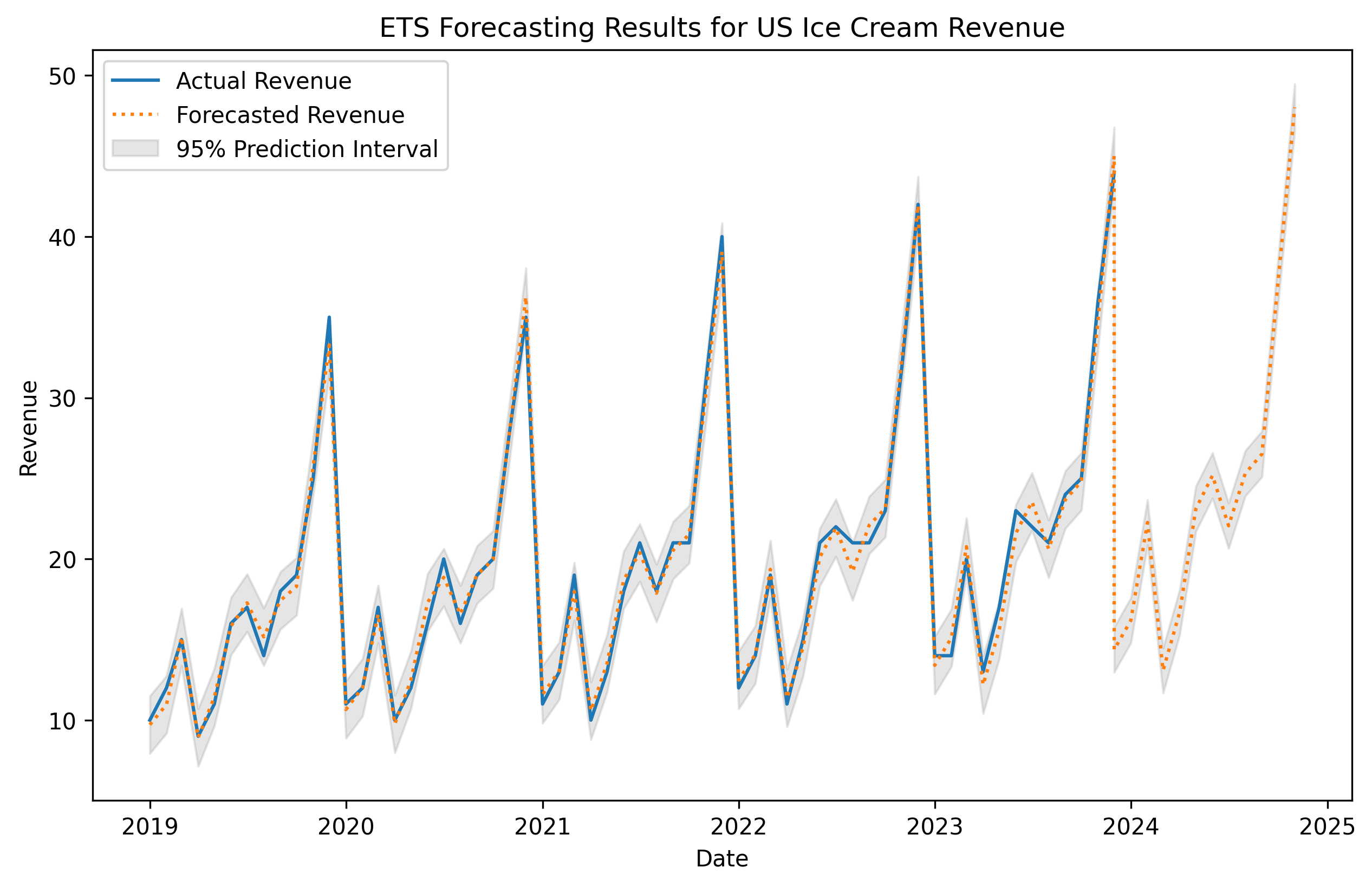
Nice! The ets model was able to capture the historical trend and seasonality and carry it forward into the future. We’re also able to see two other things in the chart.
- Hypothetical forecasts of the training data. These are often referred to as fitted values and can be used to calculate residuals, which are simply the difference between the forecast and actual value. Historically the ets model performed very well, closely matching the actual revenue values from month to month.
- A 95% prediction interval. This represents with 95% certainty the upper and lower ranges where the model thinks the future value will land between. The tighter this interval the more certain the model is in its prediction. We will dig deep into prediction intervals in more detail in a later post.
Reversal
ETS models are powerful, but not in every circumstance. Here are situations where they might struggle to produce quality forecasts.
- Big, sudden shifts (a merger, a COVID‑style shock, a new pricing policy)
- ETS learns slowly, so its forecasts keep reaching back to “the old world” and miss the new level or trend.
- Stop‑and‑go, “lumpy” demand (lots of zeros, random spikes)
- Exponential averaging smooths the spikes away, underforecasting the future.
- More than one seasonality marching at once (hour‑of‑day + day‑of‑week + holidays)
- Classic Holt‑Winters can juggle only one seasonal cycle, so leftover patterns keep showing up in the residuals.
- When outside forces rule the game (promotions, ad spend, macro shocks)
- ETS is univariate, if your forecast errors line up with random one time events, you’re in the wrong model.
- Tiny history (less than two full seasons of data)
- With so little to learn from, ETS guesses at seasonality and wobbles all over the place.
Final Thoughts
ETS shines when your data marches to one clear seasonal drumbeat and drifts in a steady direction. Feed it that steady history and it returns forecasts that are fast, transparent, and business-ready. Know its blind spots (multiple calendars, lumpy demand, sudden upheavals) and you’ll know exactly when to trust it and when to reach for heavier gear.
Learn More
- Forecasting Principles and Practice by Rob Hyndman
- ETS Models by Nixtla