This post is part of the data cleaning chapter within a larger learning series around time series forecasting fundamentals. Check out the main learning path to see other posts in the series.
The example monthly data used in this series can be found here. You can also find the python code used in this post here.
Keeping It In Between The Lines
Most of time series forecasting is all about trying to fit a line to your data. There are a million ways to do it, but at its core we want to fit a line that’s as close as possible to the original data and where we think future data points might lie.
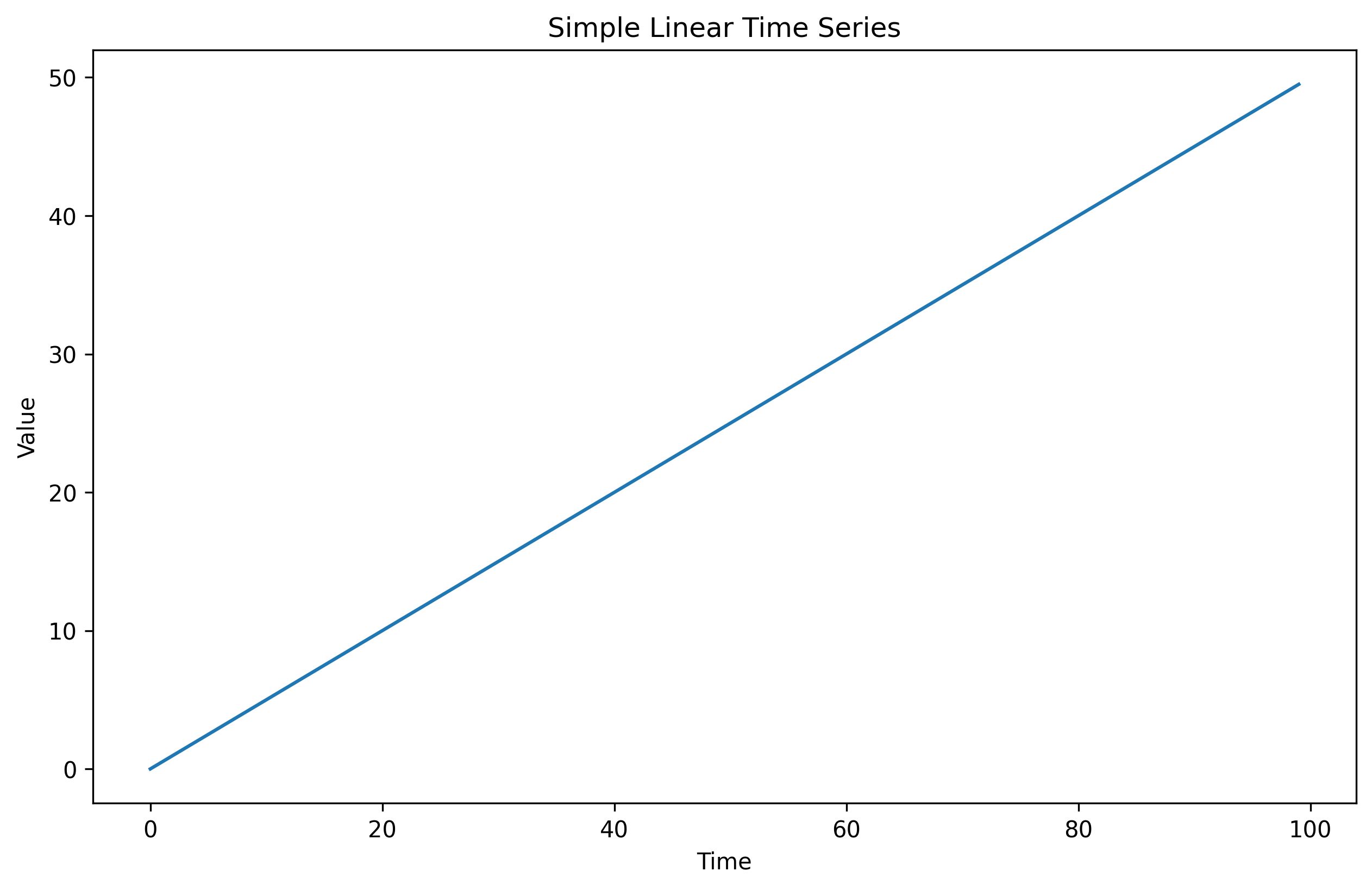
The easiest line to fit is already a straight line, or one that has linear growth. Consider the chart below. What do you think the future forecast will be? Pretty easy, a model can just extend the same upward linear growth going forward.
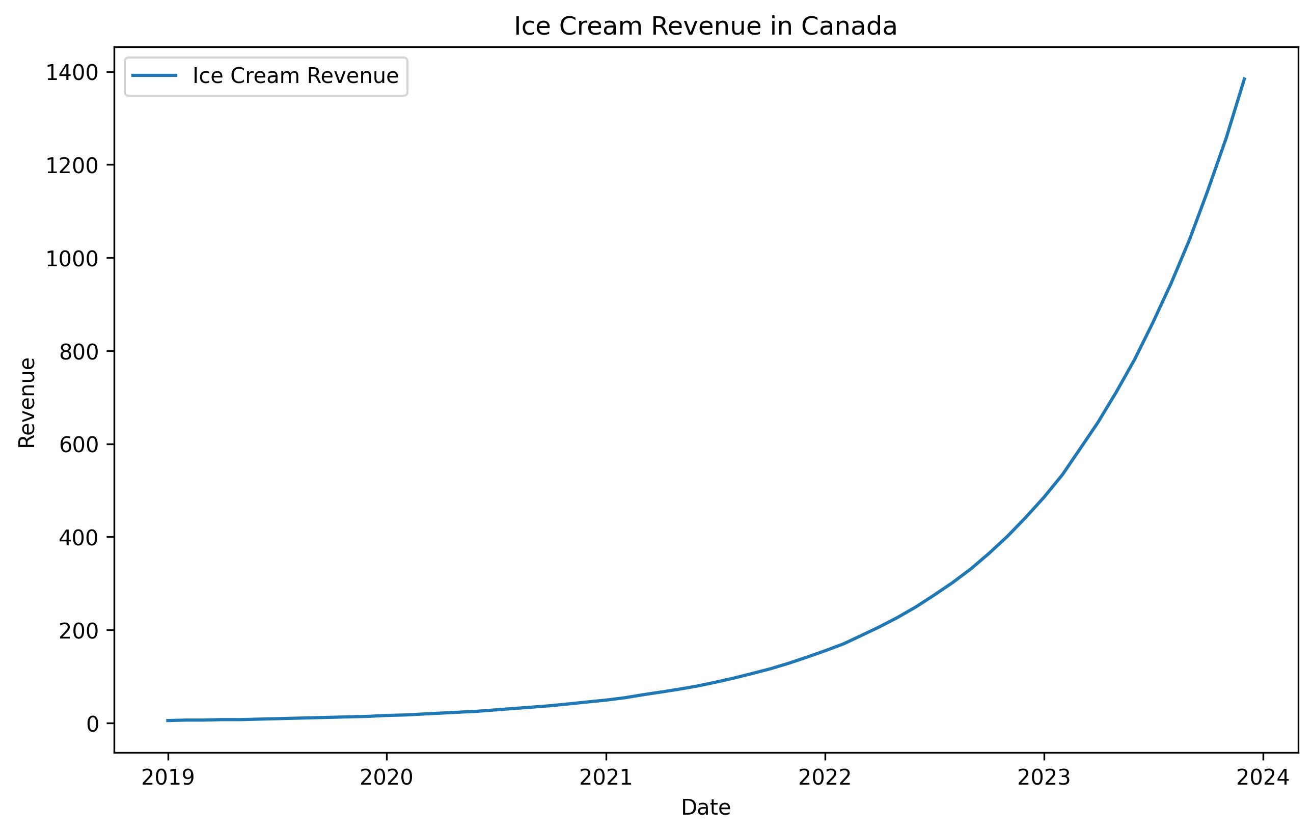
We would always prefer to model a time series that has a linear trend. But often that’s not the case in businesses. Revenue might double every year, and that my friend is not a linear line, but instead an exponential one. A time series growing exponentially is harder for many models to forecast because most models expect the variance of the data to stay the same over time (more on this in the stationary post), and a expanding time series violates this assumption. Consider one of our example time series in our dataset below. See how it grows not at a linear pace but a hockey stick like exponential pace?
A good way to handle this exponential growth is to transform it into one that looks more linear. This is where a technique called a box-cox transformation comes in handy.
Box-Cox Enters The Chat
The Box-Cox transformation is a family of power transformations that aim to make data more normally distributed and stabilize its variance. In simple terms, it transforms your original values using an exponent (λ, “lambda”) to reduce skewness.
Lambda can take many values. A lambda of 0 corresponds to a log transform. A value of 0.5 is a square root transform. By transforming our data this way we can in essence de-scale the data to ensure any large spikes are dampened and easier for a model to fit the data. This can transform our data to be homoscedastic, or having constant variance. Let’s see how our time series looks after applying a few box-cox transformations.
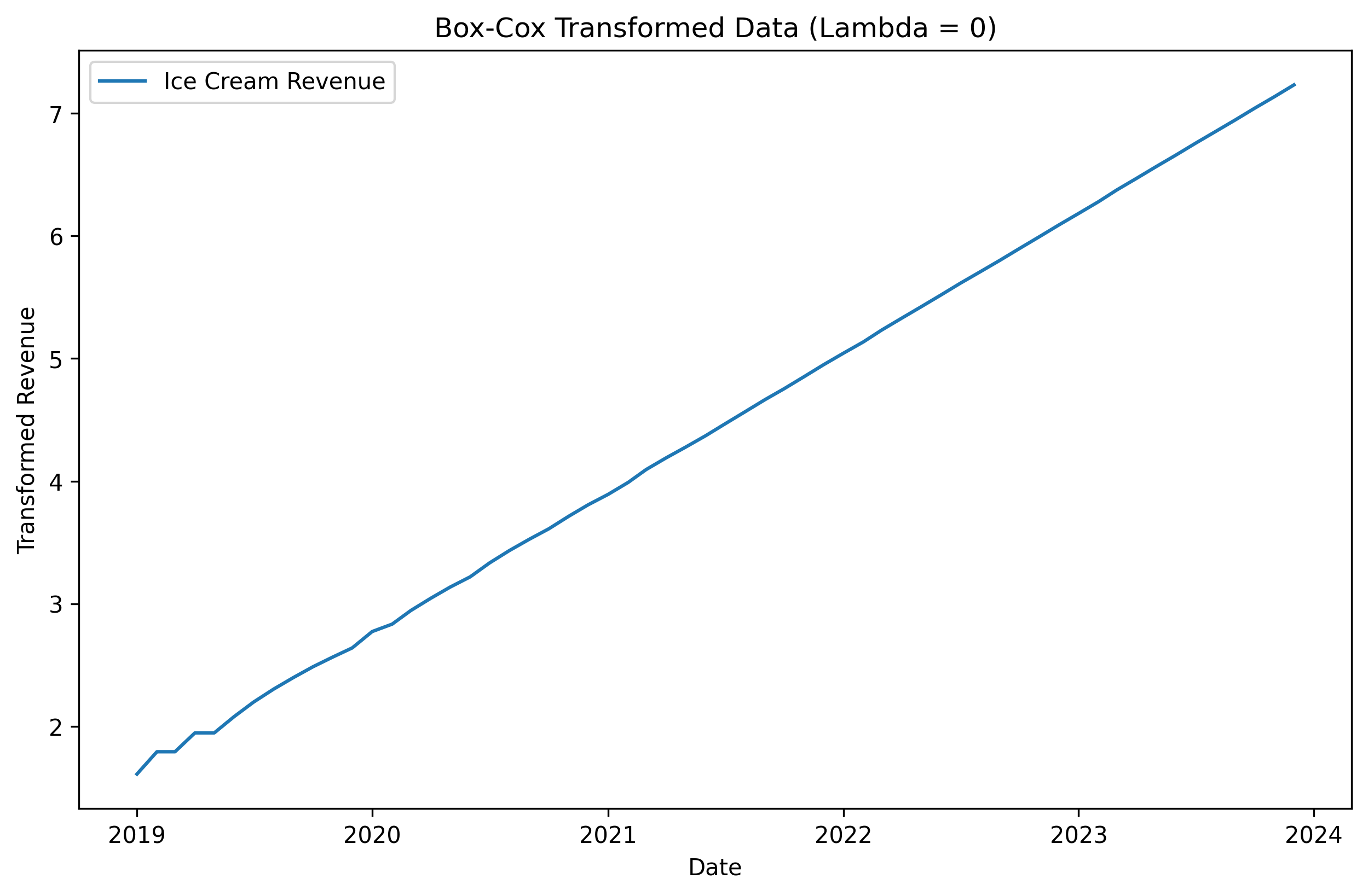
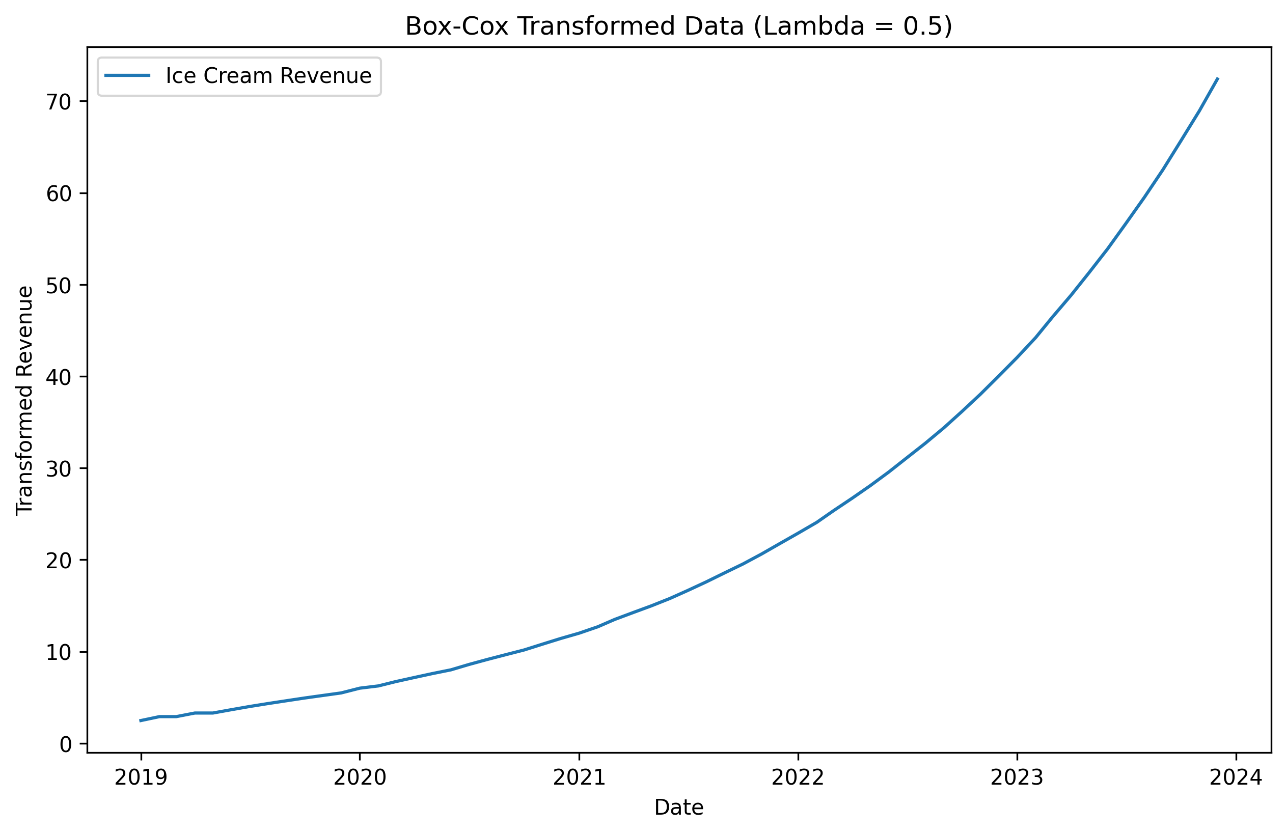
The log transformation (lambda = 0) seems to have done a great job at turning our exponential growth into linear growth. The square root transformation (lambda = 0.5) didn’t do as well. Choosing the right value of lambda is important, thankfully there is an automated process that can do it for us. Let’s see how the data looks with an optimal lambda value chosen automatically.
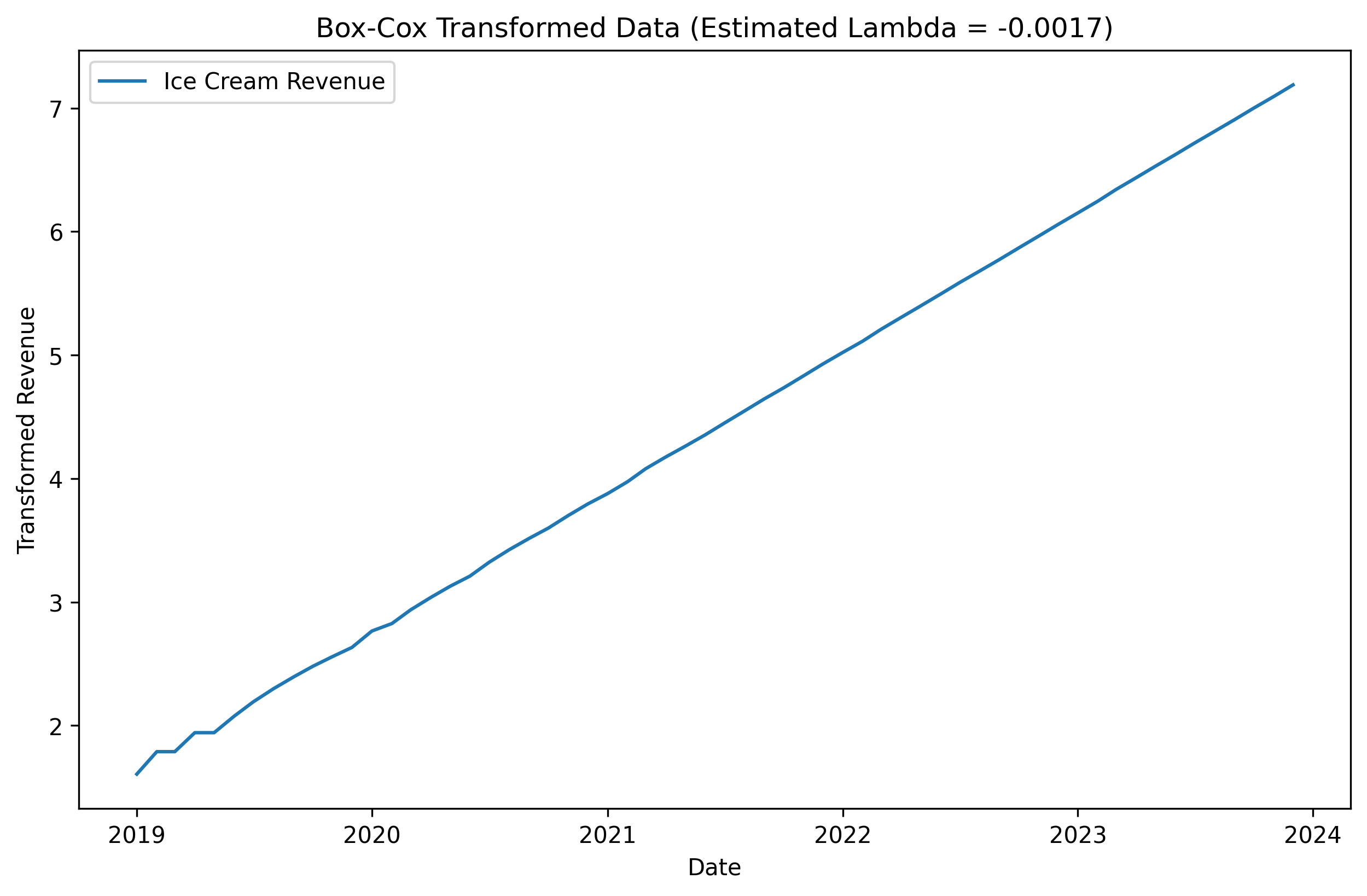
The automated process chose a lambda value very close to zero. So it basically did a simple log transformation. Now our data has become much easier to model correctly, how cool is that!
Reversal
There are no perfect solutions, only tradeoffs. Here are a few when using box-cox transformations.
- Runaway exponential trends: If your time series has exponential trend aspects, but isn’t actually a true exponential trend, there can be big repercussions. A model might take that transformed data and start creating future forecasts that are astronomical in size, going from thousands to trillions in a few periods. A good example is a time series that is stable for most of its history, then at the very end it all of a sudden has tripled in value over one or two periods. A box-cox transformation will pick up on this and transform the data in a way that a model might pick up on as a trend that should grow into the future. So each subsequent forecast period might continue to triple in value. That’s not good.
- Time series can’t be zero or negative: All zero values must be changed to be a placeholder value like 0.1 or 1, that way things like a log transformation can work. There also can’t be any negative values, again because you can’t take the log of a negative number, which in some time series is unavoidable.
- Need to back transform the data after forecasting: After you train a model and create a forecast on the transformed data, you must transform the forecast back to the original units. So you have to make sure you keep the lambda value used in the box-cox transformation handy, because you will need it to inverse the transformation.
- Less model interpretability: Because a model is learning on transformed data, being able to explain the models decisions become harder. Know there is always a tradeoff between model accuracy and model interpretability.
Final Thoughts
Box-Cox transformations are a powerful tool for taming exponential growth in time series, making trends easier to model and forecast. However, like any transformation, they come with tradeoffs. Potentially misleading trends, the need for careful handling of zeros and negatives, and additional steps to back-transform predictions. Despite these challenges, applying box-cox correctly can make a significant difference in forecasting accuracy. The key takeaway? Use transformations thoughtfully, always validate their impact on your specific dataset, and remember that the best forecast starts with well-prepared data.