
Time Series First Principles Series
This post dives into the ninth principle of a good time series forecast, model combinations are king. Check out the initial post in this series to get a high level view of each principle.
Wisdom of the Crowds
In 1906, famed statistician Francis Galton went to a county fair for some fun. While there he came upon a competition to guess the weight of an ox. Eight hundred people entered the competition but the guesses were all over the place, some too high, some too low. Francis was a big numbers guy, so he took all of the guesses home with him and crunched the data. He found out that the average of all the guesses was only one pound away from the actual weight of the ox, which weighed 1,198 pounds. That’s an error of less than 0.08%. What he stumbled upon that day is now know as the wisdom of the crowds.
The concept of wisdom of the crowds states that the collective wisdom of a group of individuals is usually more accurate than that of a single expert. When guessing the weight of the ox, the overestimates and underestimates of regular people cancelled each other out. Creating an average prediction that was more accurate and any single person’s estimate.
This principle is important in machine learning forecasting. Usually it’s not one single model that performs the best, but instead a combination of multiple models. Let’s take a look at how we can combine models into more accurate forecasts.
Types of Model Combinations
There are many different ways individual model forecasts can be combined to create more accurate forecasts. For today we’ll cover the most common approaches. If you’d like to dive deeper I recommend this amazing paper by our forecasting Godfather Rob Hyndman.
- Simple Average: As simple as it sounds. Just take the forecasts from individual models and average them together.
- Ensemble Models: Feed the individual model forecasts as features into a machine learning model, and have the model come up with the correct weighted combination. This is also known as “model stacking”.
- Hierarchical Reconciliation: This involves forecasting at different aggregations of the data set based on its inherent hierarchies, then reconciling the down to the lowest level (bottoms up) using a statistical process. For example forecasting by city, country, continent, and global level then reconciling each forecast down to the city level. This reconciliation can be thought as combining different forecasts together to create something more accurate. This approach has more nuances, and will be covered in another post.
Model Combination Example
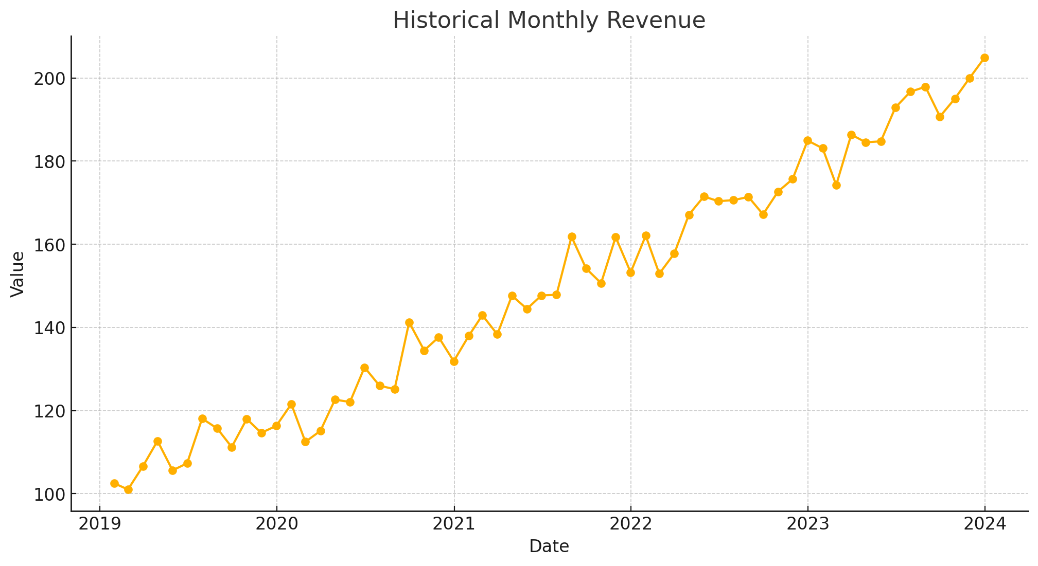
Let’s walk through a simple example around how combining the predictions of more than one model can outperform any single model. Below is an example monthly time series. We will try to back test the last 12 months of the historical data.
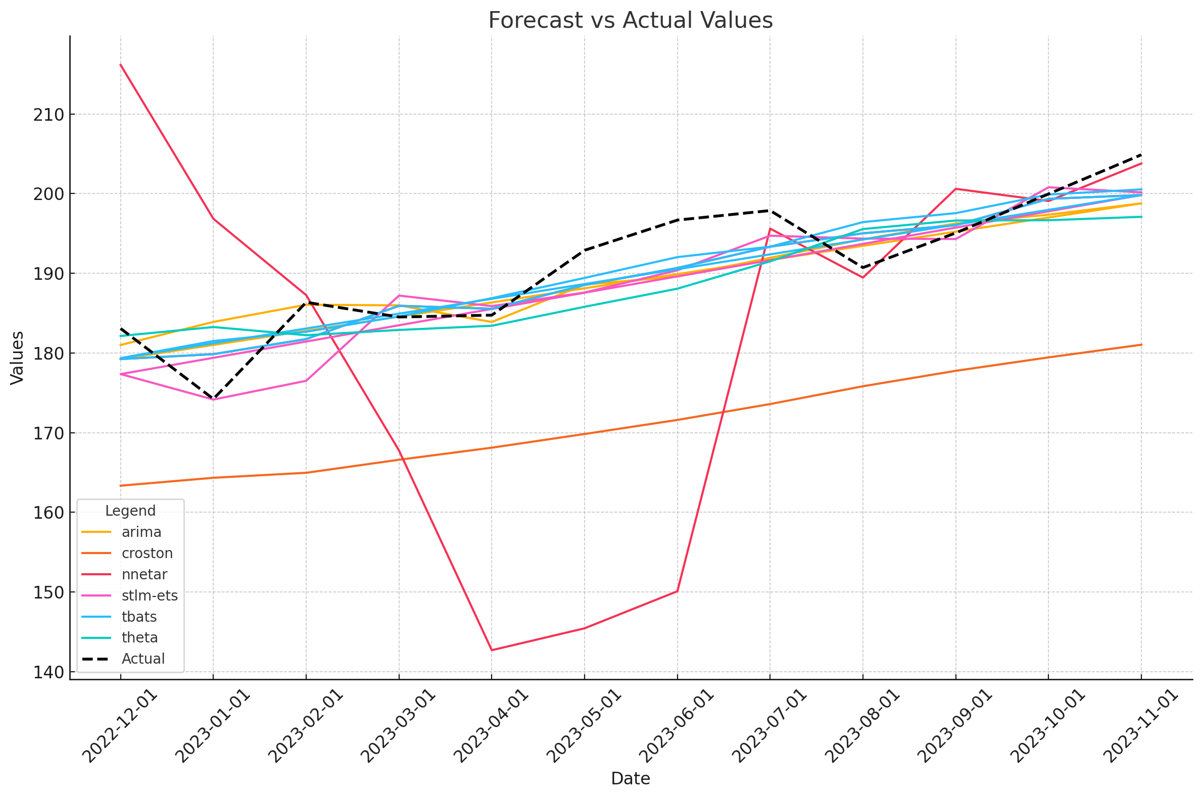
To keep things simple we can just run a few models to get the back testing results for the last year of the data. We’ll use various univariate time series models. Ignore the types of models used. Instead, let’s just see how each model did on it’s own. Learn more about accuracy metrics in a previous post.
| Model | MAPE | MAE | RMSE |
|---|---|---|---|
| arima | 1.97 | 3.76 | 4.68 |
| croston | 10.18 | 19.54 | 20.01 |
| nnetar | 9.77 | 18.37 | 26.00 |
| stlm-ets | 1.92 | 3.68 | 4.59 |
| tbats | 1.86 | 3.51 | 4.05 |
| theta | 2.46 | 4.71 | 5.52 |
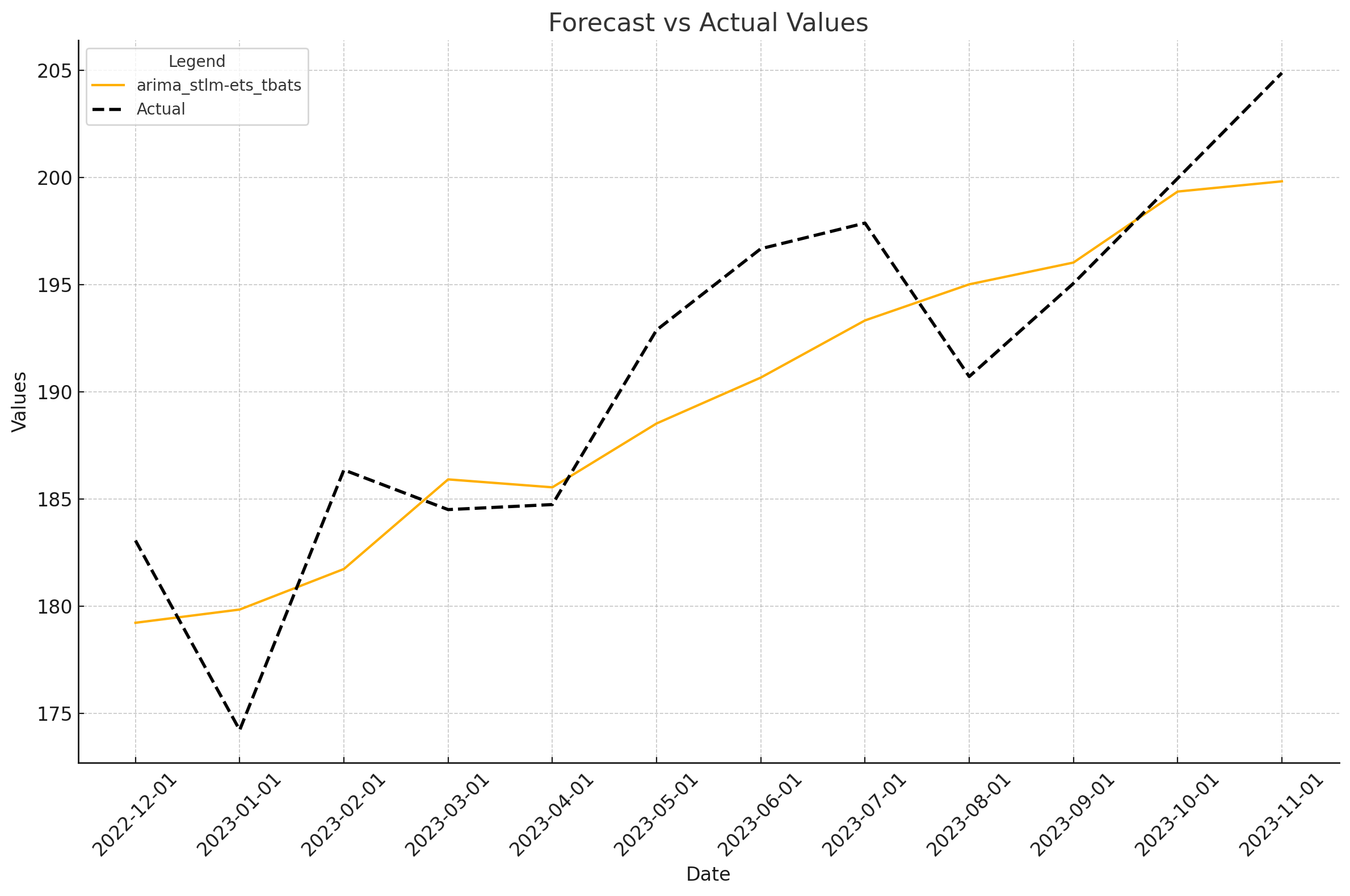
It looks like the tbats model performs the best across the board with stlm-ets and arima not far behind. What if we averaged the three of them together? Let’s see how the results change.
| Model | MAPE | MAE | RMSE |
|---|---|---|---|
| arima_stlm-ets_tbats | 1.84 | 3.51 | 3.99 |
Even better results! See how creating simple model averages can improve the results? Averaging the results can help smooth out any under or over forecasts, creating more accurate models.
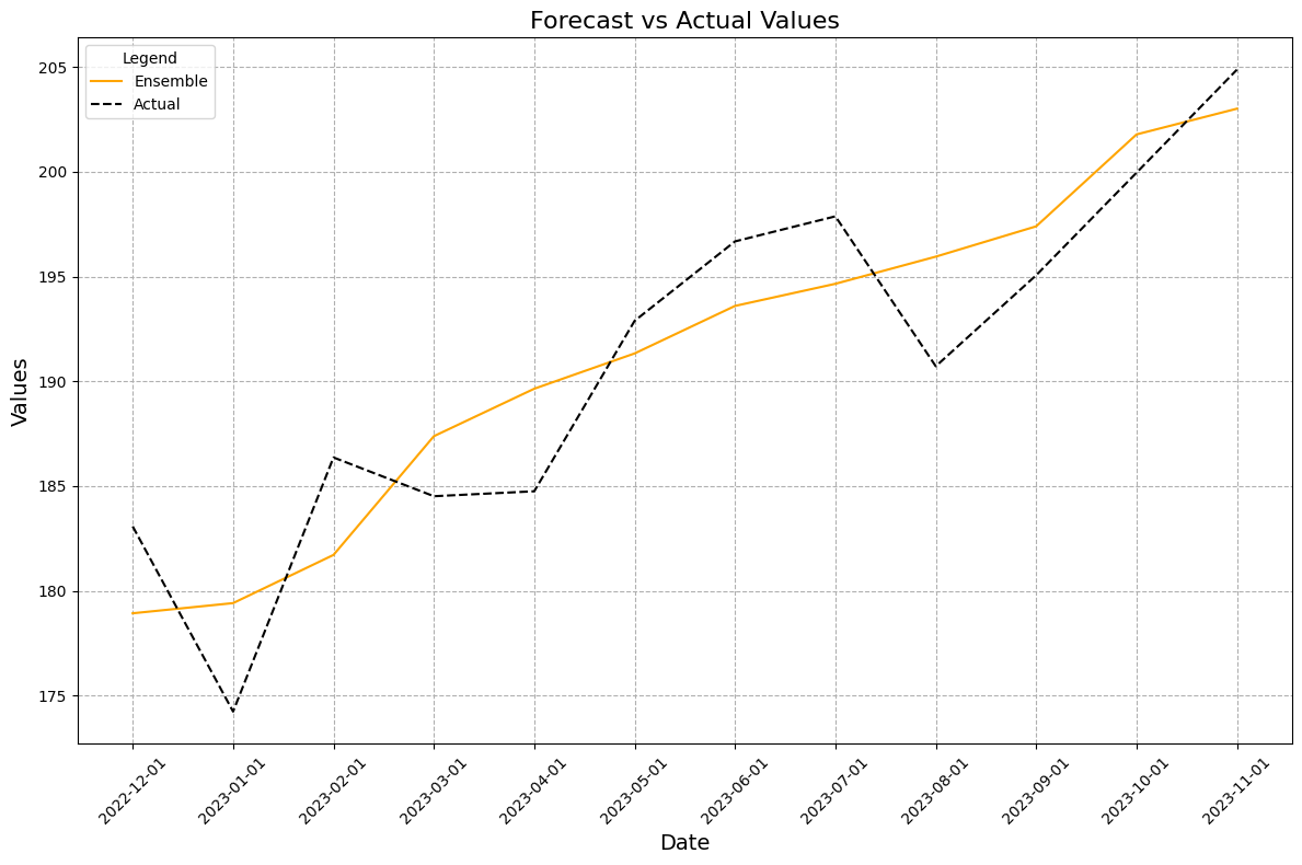
Simple model averages are often the quickest way to improved forecast accuracy. Another way is to create an ensemble model that can create the weights on its own. Let’s feed the predictions from each model into a linear regression model and have it determine the optimal weights.
| Model | MAPE | MAE | RMSE |
|---|---|---|---|
| Ensemble | 1.81 | 3.40 | 3.65 |
Alight more accurate results! By feeding each individual model forecast into a final ensemble model, we were able to get a more accurate forecast.
Reversal
When trying to combine models, there is always a risk of overfitting. Meaning the combination approach (like simple average or ensemble) could have great accuracy on the back test data but not generalize well to new unseen data in our future forecast. To prevent that we can make sure to back test on enough historical data to prove our combination approach works well for more than just a period or two. We can also have separate validation and test splits in the back testing to see how combinations made on one data set can generalize well when tested on the other.
Prediction intervals are harder to create. Simply combining the 80% and 95% prediction intervals of multiple models together is not going to fully capture the uncertainty of forecasts created by the new model combination. So we would need to re-create the intervals based on the results of the new combined model.
Similar to prediction intervals, combining models can also make it harder to interpret them. Instead of just understanding one model and its predictions, we now have to understand how multiple models work and are combined to get the final forecast.
finnts
Model combinations can be hard to do effectively. Thankfully my forecasting package, finnts, is here to help! It automatically handles every kind of model combination method listed in this post. Check out the package and see just how easy forecasting can be.
Final Thoughts
Just like the county fair crowd nailed the ox’s weight, combining multiple models in time series forecasting yields more accurate predictions by balancing out individual errors. When you’re forecasting, remember to embrace the collective wisdom of models for better results!